# MPM 水# 简介 对于流体模拟来说有两种视界,一种是拉格朗日视角一种是欧拉视角,
拉格朗日视角就是把物理量存在粒子上,因为粒子是自由移动,所以很容易做 advection,做起动量守恒很容易,但粒子是离散化,使得检测周围邻居变得异常困难,但可以用哈希结构数据储存来检索,就像 niagara neighbor 3d 欧拉视角则是把世界分为一个个 grid,所有物理量在都是在 Grid 上,因为是 Grid 所以很容易求出 Projection,就是压强,但欧拉 grid 面对 advection 很难,模拟的时候回流能量损失,流体看起来非常粘 而 MPM 质点法就是混合了拉格朗日视角和欧拉视角,他由 FLIP 方法的扩展而提出的,FLIP 就是现在官方 Niagara 中所使用的模拟方法。而 MPM 的好处是实现起来很简单,可以模拟各种离散材料,并且可以让他们互相作用,例如水和沙子之间互相作用,或者 softbody 和 water 和雪之间的互相作用,在模拟水这一块,FLIP 用的是隐式积分,要几十次迭代求解压力场才能收敛,而且需要求多个 Grid 求 Δ,MPM 在运行速率比 FLIP 的快一点。
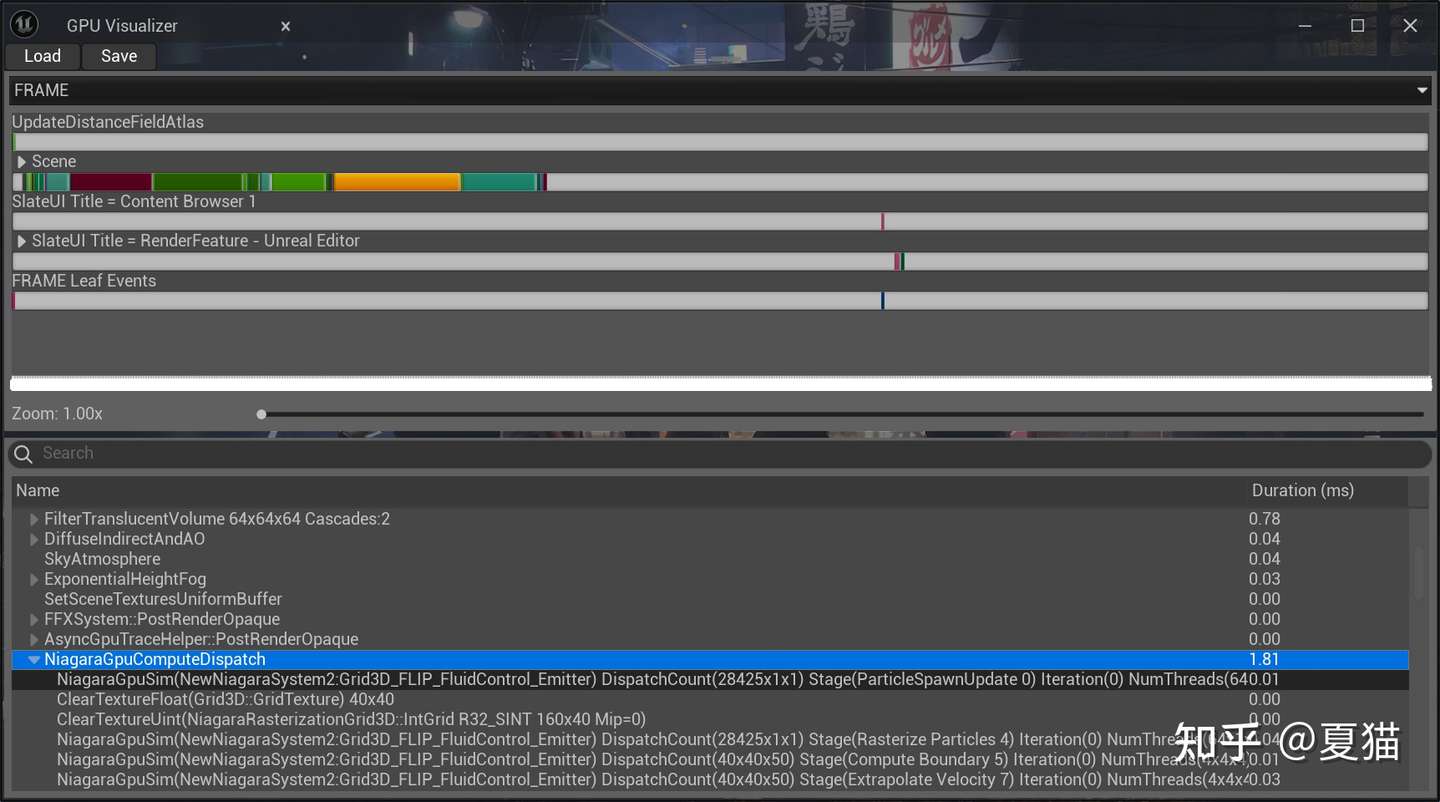
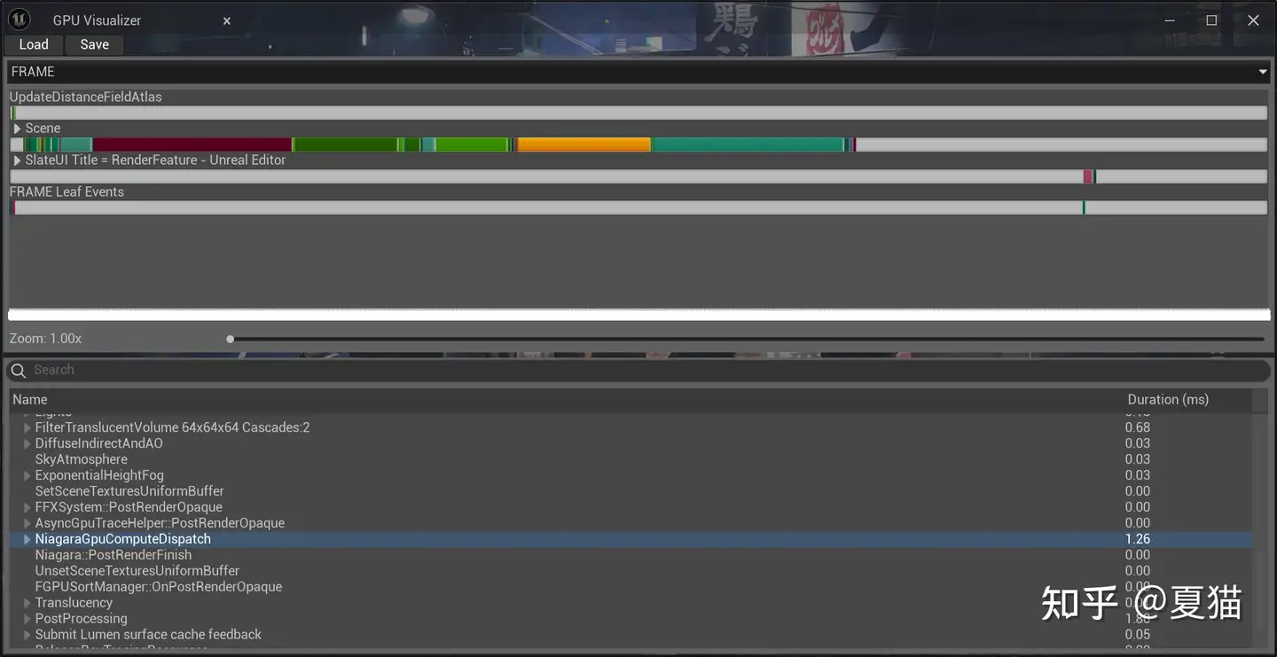
测试两个系统同时运行一秒后,在 50 个格子的精度下,spawn rate 是 20000 情况下,压力场迭代 200 次官方水是 1.81 秒,MLS-MPM 是 1.26 秒
官方 FLIP 水
# MPM PIC(particle in cell)是在 MPM 框架下最初提出来的 method,MPM simulation 大致实现的步骤就是先把粒子插值分配到周围 Grid 上(particle to grid),然后在 Grid 上计算力和各种互相作用力,然后再插值回粒子求出速度( grid to particle)
# PIC - Particle In Cell 先把粒子通过 B-Spline 插值到 3x3,一般就是用 Quadratic 足够 smooth
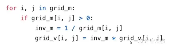
这是代码,看起来简单明了,这个过程就叫 P2G,其中插值不是以当前点为中心,而且粒子点所在的 3x3 区块的右下角,所以 base 才有 - 0.5
然后 Grid 上动量除于 Mass 就是速度了
最后把网格速度重新收集到粒子上,再 B-Spline 插值回去
但是这个 method 有个问题就是有能量损耗,,平移没有耗散,但拉式,旋转,剪切都是有耗散的,运动一会就不动了,原因是信息的丢失,在原来二维的 Grid 上有 18 个自由度,3x3 个格子和各个 xy,但传播到粒子上就只有两个自由度,就是只有 xy。
解决办法就是给粒子记录更多信息,就是 APIC,多了一 C 矩阵,记录 x y 方向的拉伸、剪切旋转量、剪切量
还有个方法就是只传输 Δx 信息,就是对格子求导得到最终速度给粒子,就是 FLIP
# APIC-affine particle in cell 先看看 particle to grid 的公式,
将每个粒子的质量分配到该粒子周围的网格上,并使用粒子的速度及 affine 矩阵计算每个网格的速度。
( m v ) i n + 1 = ∑ p w i , p [ m p v p n + m p C p n ( x i − x p n ) ] (m\textbf{v} )_i^{n+1}=\sum_pw_{i,p} [m_p \textbf{v}_p^{n}+m_p\textbf{C}_p^n(\textbf{x}_i-\textbf{x}_p^n)] ( m v ) i n + 1 = p ∑ w i , p [ m p v p n + m p C p n ( x i − x p n ) ]
m i n + 1 = ∑ p m p w i , p m_i^{n+1}=\sum_pm_pw_{i,p} m i n + 1 = p ∑ m p w i , p
其中, w i , p w_{i,p} w i , p p p p i i i C p n \textbf{C}_p^n C p n p p p i i i x i \textbf{x}_i x i
对于 APIC 的实现公式很简单,但其推导及其复杂,所以就不写推导了
APIC 在 PIC 上多加了一个矩阵和 affine
然后 Grid to Particle 公式就是下面,同时为每个粒子计算 affine 矩阵。
v p n + 1 = ∑ i w i , p v i n + 1 C p n + 1 = 4 Δ x 2 ∑ i w i , p v i n + 1 ( x i − x p n ) T x p n + 1 = x p n + Δ t v p n + 1 \textbf{v}_p^{n+1}=\sum_iw_{i,p}\textbf{v}_i^{n+1} \\\textbf{C}_p^{n+1}=\frac{4}{\Delta x^2}\sum_iw_{i,p}\textbf{v}_i^{n+1}(\textbf x_i-\textbf x_p^n)^{\textbf T} \\\textbf{x}_p^{n+1}=\textbf{x}_p^n+\Delta t \textbf{v}_p^{n+1} \\ v p n + 1 = i ∑ w i , p v i n + 1 C p n + 1 = Δ x 2 4 i ∑ w i , p v i n + 1 ( x i − x p n ) T x p n + 1 = x p n + Δ t v p n + 1
v i n + 1 ( x i − x p n ) T \textbf{v}_i^{n+1}(\textbf x_i-\textbf x_p^n)^{\textbf T} v i n + 1 ( x i − x p n ) T
这是 APIC 论文,有兴趣可以读读
https://www.math.ucla.edu/~cffjiang/research/apic/paper.pdf
# MLS-MPM 那么现在就到本文在 Niagara 实现的方法,就是在 APIC 上进行了改进,在 APIC 上多了个 stress,称为 Cauchy Stress,起到的作用是表现抵抗压缩的力,在 P2G 公式是这样的
F p n + 1 = ( I + Δ t C p n ) F p n ( m v ) i n = ∑ p w i , p { m p v p n + [ m p C p n − 4 Δ t Δ x 2 ∑ p V p 0 P ( F p n + 1 ) ( F p n + 1 ) T ] ( x i − x p n ) } m i n + 1 = ∑ p m p w i , j \textbf{F}_p^{n+1}=(\textbf I+\Delta t \textbf C_p^n)\textbf{F}_p^{n} \\(m\textbf v)_i^{n}=\sum_pw_{i,p} \left\{ m_p \textbf v_p^n+\left[m_p\textbf C_p^n-\frac{4\Delta t}{\Delta x^2}\sum_p V_p^0\textbf P(\textbf F_p^{n+1})(\textbf F_p^{n+1})^T \right](\textbf x_i-\textbf x_p^n)\right\}\\ m_i^{n+1}=\sum_pm_pw_{i,j}\\ F p n + 1 = ( I + Δ t C p n ) F p n ( m v ) i n = p ∑ w i , p { m p v p n + [ m p C p n − Δ x 2 4 Δ t p ∑ V p 0 P ( F p n + 1 ) ( F p n + 1 ) T ] ( x i − x p n ) } m i n + 1 = p ∑ m p w i , j
其中,F p n \textbf F_p^n F p n P ( F p n ) \textbf P(\textbf F_p^{n}) P ( F p n )
# MLS-MPM 公式推导 那么中间那一项是怎么得出来的呢,首先要求出当前点的动量,那么该点所受到一定是冲量叠加上去的,假设我们用超弹性材料模型
而所受到的的力就是总体弹性势能求导,其中 ψ p \psi_p ψ p V p V_p V p
假设我们 Particle 向前移动 τ \tau τ τ \tau τ V i V_i V i τ \tau τ τ \tau τ
这是 MLS-MPM 原论文,由胡渊鸣 大佬写的,也可以看一下 Games201
# Niagara 实现 从上面可以知道 MLS-MPM 是实现起来非常简单,运行性能也很快,所以在 Niagara 实现也很简洁
首先是设置 Grid3d,这里要用到原子操作,所以要用到 Rasterization Grid3D,这里有很奇怪的 bug,在跑 Rasterization Grid3D 一定要带 Grid3D 一起玩,否则粒子动一下就不动了。
因为要把速度和质量写入 grid3d,所以 RasGrid 的 NumAttribute 要开 4 个,我写 7 个是因为还要把颜色写入可以做不同发射源做颜色混合。
# initial
# P2G 然后做 P2G 操作,这里我写了个很傻的模组,就是把粒子 trasform 到 Grid 空间,就是把位置和速度归化 0-1,因为我们是显示积分,要是用世界位置的话,一下子数字就 inf 就炸开了,在官方有个 module 可以直接用来算矩阵然后 mul position 就行了
在流体模拟里面,形变矩阵 F 会随着时间变得越来越大,但模拟到一定时候后,float 这时候精度就不够用了,为了解决问题,在 A.P Tampubolon et al. (2017) 这篇文章中我们可以用 F 的行列式来表示整个矩阵的变化,这时候我们就可以用去记录 F,用 J 来代替,J 的定义如下。其中矩阵 C 对体积有贡献的只有对角线,所以就用 C 的迹
1
2
3
4
5
6
7
8
9
10
11
12
13
14
15
16
17
18
19
20
21
22
23
24
25
26
27
28
29
30
31
32
33
34
35
36
37
38
39
40
41
42
43
44
45
46
47
48
49
50
51
52
53
54
55
56
57
58
59
60
61
62
63
64
65
66
int Cellx;int Celly;int Cellz;float dx = 1 /(float )Cellx;0.5 );3 ];float IGNORE ;0 ] = 0.5 * (1.5 - FPosition) * (1.5 - FPosition);1 ] = 0.75 - (FPosition - 1 ) * (FPosition - 1 );2 ] = 0.5 * (FPosition - 0.5 ) * (FPosition - 0.5 );float DeltaDx = dx*dx;float pvol = pow (dx*0.5 ,3 );1 + DeltaTime * (C[0 ][0 ] + C[1 ][1 ] + C[2 ][2 ]));float Stress = -DeltaTime * 4.0 * E * pvol * (J - 1 ) / DeltaDx;0 ,0 ,0 ,0 ,Stress,0 ,0 ,0 ,0 ,Stress,0 ,0 ,0 ,0 ,0 for (int x = 0 ;x<3 ;x++)for (int y = 0 ; y < 3 ; y++)for (int z = 0 ; z<3 ; z++)int IndexX = BasePosition.x + offset.x;int IndexY = BasePosition.y + offset.y;int IndexZ = BasePosition.z + offset.z;if (IndexX < Cellx&&IndexY < Celly&&IndexZ < Cellz&&0 &&IndexY > 0 &&IndexZ > 0 )float CellWeight = Weight[x].x*Weight[y].y*Weight[z].z;0 ;0 );float GridMass ;//= GridData.w;0 , GridVelocity.x,IGNORE);1 , GridVelocity.y,IGNORE);2 , GridVelocity.z,IGNORE);3 , GridMass,IGNORE);4 ,Color.x *CellWeight ,IGNORE);5 , Color.y *CellWeight,IGNORE);6 , Color.z *CellWeight,IGNORE);0 , float4(GridVelocity,GridMass));
# G2P 因为我没有做什么其他物质之间的交互,所以我们省略中间对 Grid 的操作,还有一点就是我不知道为什么单独操作 Rasterization Grid3D, 值是 0,所以我放弃这一个,直接合到 G2P 过程,并且在这里做 Bound 操作
1
2
3
4
5
6
7
8
9
10
11
12
13
14
15
16
17
18
19
20
21
22
23
24
25
26
27
28
29
30
31
32
33
34
35
36
37
38
39
40
41
42
43
44
45
46
47
48
49
50
51
52
53
54
55
56
57
58
59
60
61
62
63
64
65
66
67
68
69
70
71
72
73
74
75
76
77
78
79
80
81
82
83
84
85
86
87
88
89
90
91
92
93
94
95
96
97
98
99
100
101
102
103
104
105
106
107
108
109
110
111
112
113
114
115
116
117
118
119
int Cellx;int Celly;int Cellz;float dx = 1 /(float )Cellx; //(float )Cellx / WorldSize.x;0.5 );3 ];0 ] = 0.5 * (1.5 - FPosition) * (1.5 - FPosition);1 ] = 0.75 - (FPosition - 1 ) * (FPosition - 1 );2 ] = 0.5 * (FPosition - 0.5 ) * (FPosition - 0.5 );float DeltaDx = dx * dx;0 ;0 ;0 ;for (int x = 0 ;x<3 ;x++)for (int y = 0 ; y < 3 ; y++)for (int z = 0 ; z<3 ; z++)int IndexX = BasePosition.x + offset.x;int IndexY = BasePosition.y + offset.y;int IndexZ = BasePosition.z + offset.z;if (IndexX < Cellx&&IndexY < Celly&&IndexZ < Cellz&&0 &&IndexY > 0 &&IndexZ > 0 )float CellWeight = Weight[x].x*Weight[y].y*Weight[z].z;0 , GridData);0 , GridData.x);1 , GridData.y);2 , GridData.z);3 , GridData.w);0 ;4 , TempColor.x);5 , TempColor.y);6 , TempColor.z);if (GridData.w > 0 )float DistanceToNearestSurface;bool IsDistanceFieldValid;if (IndexX > Cellx - Bound && GridData.x > 0 )if (IndexX < Bound && GridData.x < 0 )if (IndexY > Celly - Bound && GridData.y > 0 )if (IndexY < Bound && GridData.y < 0 )if (IndexZ > Cellz - Bound && GridData.z > 0 )0 ;if (IndexZ < Bound && GridData.z < 0 )0 ;if (IsDistanceFieldValid&&DistanceToNearestSurface <3 )0.9 ;1 )*length(GridData.xyz)*1.5 ;0 ,0 ,0 ,0 ,0 ,0 ,0 4 * CellWeight * GOuterProduct / DeltaDx;0.01 ));float colF1 = length(C[0 ]);float colF2 = length(C[1 ]);float colF3 = length(C[2 ]);float Fa = length(float3(colF1,colF2,colF3));if (Fa >50 )2. f;for (int i = 0 ;i<4 ;i++)for (int j = 0 ;j < 4 ; j++)10 ,10 );98. f;